Fractional Taylor Series

Home Up Back Leave Message

(WIP)
(Please note this first part will eventually be moved out to its own section on fractional calculus, it is just provided here as an introduction on doing Taylor series with fractional calculus)
Let's have a look at something different. In normal calculus we differentatiate in integral steps. Thus if we take the following:

$$ \begin{aligned} {dx \over dy} = f^{(1)}\\ {{d^2x} \over {dy^2}} = f{(2)}\\ \cdots\\ {{d^nx} \over {dy^n}} = f{(n)}\\ \end{aligned} $$

From this we can see that the nowhere do we have something like $f^{(1.23)}$ which would mean a fractional derivative which is not handled by standard calculus.

Polynomial Fractional Derivatives

The integral derivatives of $f(x) = x^n$ is as follows:

$$ \begin{aligned} f^{(1)}(x) & = n*x^{n-1}\\ f^{(2)}(x) & = n*(n-1)*x^{n-2}\\ f^{(3)}(x) & = n*(n-1)*(n-2)*x^{n-3}\\ \cdots\\\ f^{(m)}(x) & = n*(n-1)*(n-2)\cdots(n-m+1)*x^{n-m}\\ \end{aligned} $$

This we can write more compactly as:

$$ \begin{aligned} f^{(m)}(x) & = {{n!}\over{(n-m})!} * x^{n-m}\\ \end{aligned} $$

This was now for integer cases of $m$ but nothing stops us to have a look at fractional (or decimal) and complex values of $m$. The only thing we need to do is replace $n!$ with $\Gamma(n+1)$ where $\Gamma$ is the gamma function (see Wikipedia for a more indepth discussion). This can be determined by the following

$$ \begin{aligned} \Gamma(z) = \int_0^\infty x^{z-1}e^{-x} dx \end{aligned} $$

This is a bit of a difficult thing to calculate and it is therefore done by numeric means. But for us it is just important it can be done.

We can now rewrite above case to:

$$ \begin{aligned} f^{(m)} (x) & = {{\Gamma(n+1)}\over{\Gamma(n-m+1)}} * x^{n-m}\\ \end{aligned} $$

Where m can be a decimal or complex value.

Please see Wikipedia for a deeper discussion (with fractional integration included as well). A book covering how to approach Fractional Calculus numerically and how to apply it in engineering is Numerical Methods for Fractional Calculus, CRC Press, Zeng F. and Li C., ISBN: 978-1-4822-5381-8

Fractional derivate on Taylor series

This was now just the intro. We can use this now with Taylor series. Once we have Taylor series we can get the fractional derivative. Let start with something straight forward like $e^x$. The normal Taylor series for this is:

$$ \begin{aligned} e^x & = \sum_{j=0}^\infty {{x^j} \over j!}\\ \end{aligned} $$

To get a derivative of this series we just apply it to each term of the series. Let's rewrite this to get the fractional derivative for $e^x$:

$$ \begin{aligned} f^{(m)} e^x & = \sum_{j=0}^\infty {{{{\Gamma(j+1)} \over {\Gamma(j-m+1)}} x^{j-m}} \over \Gamma{(j+1)}}\\ & = \sum_{j=0}^\infty {{x^{j-m}} \over \Gamma{(j-m+1)}}\\ \end{aligned} $$

Some programming languages have the gamma function build in and we can write a function for example in the programming language julia to calculate this for us as follows:

function FDexp(x,m) 
    ans = 0.0
    for j = 0:100
        ans = ans + x^(j-m)/gamma(j-m+1)
    end
    return ans
end

We now that for integral derivatives of $e^x$ the results is just $e^x$. So for $x = 1$ we should get 2.718 or near it as possible (remember this is a numeric approximation not an exact answer). With the following piece of julia code we get the corresponding values for the derivative 0 (no derivative) to 10 steps:

for m = 0:10
    println(m," ",FDexp(1,m+0.000000001))
    # We add the small deviation seeing 
    # that the gamma function goes haywire 
    # at the exact negative integer points
end

The results are:

0 2.7182818290553925
1 2.718281828055392
2 2.718281829055392
3 2.718281827055392
4 2.718281833055393
5 2.7182818090553904
6 2.718281929055401
7 2.71828120905534
8 2.718286249055767
9 2.7182459290523444
10 2.718608809083187

So let's do it again but in steps of 0.1 instead of 1 but for 20 steps:

0.0 2.7182818290553925
0.1 2.7716857226646017
0.2 2.812214716939005
0.3 2.8395056692511136
0.4 2.8535798130114327
0.5 2.8548878358028906
0.6 2.844342309972228
0.7 2.823333172007379
0.8 2.793721937826155
0.9 2.757810608668013
1.0 2.718281828055392
1.1 2.67810784970818
1.2 2.6404273124009108
1.3 2.6083907136027267
1.4 2.584977823776912
1.5 2.5727930440187188
1.6 2.5738477906975974
1.7 2.589342245697732
1.8 2.619462031160664
1.9 2.6632082789989506
2.0 2.718281829055392

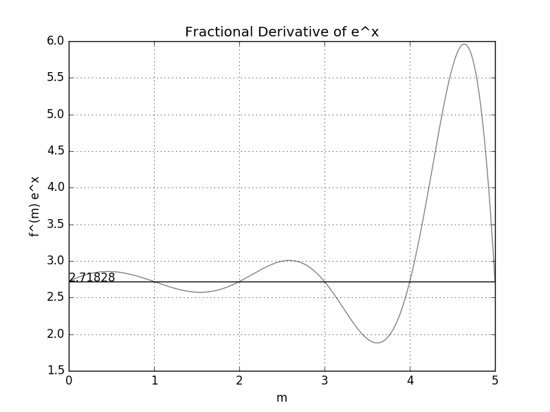
Let's see what this looks like graphically. The following image was created for 500 points from 0 to 5. One can see that the graph oscillates around the point 2.71828 (which is $e^1$, please note that x is 1 in this example that is why the graph oscillates around this point).